The purpose of this field activity was to conduct a survey using the distance and azimuth method. First, an in-class session was held to help us learn about the instruments we were going to be using. After learning about the instruments, a small survey was done right outside of the school with a partner. Later in the week it was our responsibility to conduct a survey in a different area of the University. This survey needed to include an area that was quarter-hectare plot, which is 50X50 meters. It also needed to include a total of at least 50 points.
This survey technique is used to accurately determine the
terrestrial or three-dimensional position of points and the distances and
angles between them. These points are usually on the surface of the Earth, and
are used for many applications such as creating land maps, boundaries of
ownership, building and development, mining, and etc. This method relates to
other sampling techniques, such as the point-quarter method, or mapping out
linear features on the landscape. These methods are useful for things such as
determining the population densities of individual organisms in a population or
community.
Today, new technologies, including GPS and survey stations,
allow for very accurate and precise surveying. However, you can’t always rely
on your technology coming through for you to get the job done. It’s important
to go to a job prepared for the event that your technology will fail on you.
This could happen for many different reasons including: bad weather conditions,
it could be raining or too cold for the equipment to work, the equipment may
not be charged or batteries may run out on you, the equipment might get broken
on the commute, or etc.
For this activity we were instructed to use a very basic
survey technique to map out an area. Before doing this on our own we had an
in-class session to learn about different instruments. These included a
compass, which determines azimuth, a distance finder, which calculates slope
distance, and a laser device, which determines both slope distance and azimuth
(image 1).
Image 1: Three devices presented to us in class for taking the distance
azimuth survey


Azimuth is the horizontal angle that is measured clockwise from a referent direction, as from the north, or from a referent celestial body, usually Polaris. Slope distance is the distance measured on sloping terrain that has not yet been converted to horizontal distance for plotting on a survey drawing or map. By using both azimuth and distance a surveyor can create an accurate survey of an area. However, when dealing with azimuth in surveying or navigation one must deal with the magnetic declination from true north. This should be addressed and accounted for before any surveying begins.
Magnetic Declination
Magnetic declination is the angle between compass north and
true north. Compass north is the direction the north end of a compass needle
points, while true north, is the direction along the earth's surface towards
the geographic North Pole. Magnetic declination varies both from place to place
and with time. Declination is considered positive east of true north and
negative when west. You can compute the true bearing from a magnetic bearing by
adding the magnetic declination to the magnetic bearing. For example a magnetic
declination of 10-degrees west is -10 and bearing of 45-degrees west is -45.
The National Oceanic and Atmospheric Administration (NOAA) provides a website
for calculating the magnetic declination of true north at
http://www.ngdc.noaa.gov/geomagmodels/Declination.jsp. Adjustments can be made
to the instruments you are using to compensate for magnetic declination. On
most compasses there is a screw that can be adjusted with a screw driver. For
electronic devices owner’s manuals will provide specific instructions for that
specific device.
Survey Locations
Our first survey took place right outside of the school in a
small area (image 2), where only 8 points were taken. These included 5 trees, 2
statues, and an emergency pole (images 3 and 4). This was a good area to learn how
to use the equipment because the points we were shooting at were also large and
spread out enough which made it easy to hit the targets. Another reason this
was a good spot was because the whole class was together, which made it easy to
talk to one another and ask each other questions about the instruments.
Image 2: Locational map of in-class session survey


Image 3: Two statues, emergency pole, and tree included in survey

Image 4: Four other trees included in survey

Image 5: Locational map of second survey area


Image 6: First image of panoramic view from first corner tree location
of taking survey shots

Image 7: Second image of panoramic view from first corner tree location
of taking survey shots

Image 8: Third image of panoramic view from first corner tree location
of taking survey shots

Image 9: First image of panoramic view from second corner tree location
of taking survey shots

Image 10: Second image of panoramic view from second corner tree
location of taking survey shots

Image 11: Third image of panoramic view from second corner tree
location of taking survey shots
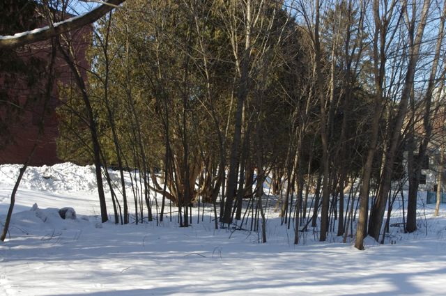
Image 12: Fourth image of panoramic view from second corner tree
location of taking survey shots

Image 13: First image of panoramic view from third corner garage
location of taking survey shots

Image 14: Second image of panoramic view from second corner garage
location of taking survey shots

Image 15: Third image of panoramic view from second corner garage
location of taking survey shots

Image 16: Fourth image of panoramic view from second corner garage
location of taking survey shots

In-class session
Before going outside to use the new equipment that was just
presented to us we had to calculate true north for Eau Claire, WI to see if any
adjustments needed to be made to our equipment. To do this our instructor went
to the NOAA website, which was presented under the magnetic declination section
in the introduction. First we entered in the zip code for Eau Claire (image
17), the longitude and latitude for Eau Claire was calculated by the website
(image 18), then it was able to compute for the declination (image 19).
Image 17: Entering Eau Claire, WI zip code to calculate for its
magnetic declination

Image 18: Calculation of Eau Claire’s longitude and latitude


Image 19: Magnetic declination calculated

Eau Claire’s magnetic declination was calculated at 0ᵒ 59’
W. Since 0ᵒ is such a small declination no adjustments to the compass or laser.
After calculating the magnetic declination we were able to
begin the survey. For this survey we were instructed to use all three
instruments we just learned about so we were familiar with how they worked.
First, my partner and I used the laser device to shoot our series of points. To
do this my partner my partner and I took turns standing by the tree we were
instructed to take our shots from (image 20).
Image 20: Taking survey shots at tree location

After taking the shot of the distance and azimuth we told one another the numbers and the other person recorded them on a piece of paper.
Our method for recording included three columns. The first column was a description of the item whose distance and azimuth was being taken, the second column included distance in meters, and the third was the azimuth. Once all 8 points were shot at and recorded with the laser device we used the distance finder and compass to take the distance and azimuth recordings. Since there were a lot of groups who needed to use the compass we both used it a few times to get the hang of it, then handed it off to another group. We already had azimuth readings from our laser. Again, we took turns using the equipment and recording the measurements.
Once the physical part of the survey was complete we went to
the computer lab and entered our recording into an Excel spreadsheet (image
21), so they could be imported into ArcMap.
Image 21: Excel Spreadsheet of survey recordings

Our Excel spreadsheet consisted of 6 columns. The first column was titled notes and contained the description of the item being recorded. The second column titled SD and contained the distance for the point with the distance finder. The third column was titled AZ and contained the azimuth of the laser device. The fourth column was titled DL and contained the recordings for the distance with the distance laser. The fifth column was titled Pt_Num and contained the number in order how the item being shot at. The Sixth column was titled X and contained contains the longitude location. Finally, the seventh column was titled Y and contained the latitude location. A few methods are possible to find the X and Y location of the tree we were shooting from. These include using a GPS, or using a high-resolution aerial image. In our case we opened up Google Earth, zoomed into the area we were surveying, put the cursor over tree we were standing at, and read the coordinates from the bottom right side of the computer screen. Lat/long were recorded in degrees with one decimal point in the degrees position. For example 91ᵒ49.96.04 W was recorded -91.499604 in the X column.
Once all the information was recorded in the spread sheet we opened ArcMap, added a base map and zoomed into the area we were surveying. Next, we created a geodatabase in ArcCatalog in our personal folder in the W drive. Once the geodatabase was created the Excel spreadsheet was imported into it. Next, we ran a tool called “Bearing Distance to Line Command”. This tool creates a new feature class containing geodetic line features constructed based on the values in an X-coordinate field, a Y-coordinated field, a bearing field, and a distance field of a table. This tool is located in ArcMap toolbox, under Data Management, and then Features (image 22).
Image 22: Location of “Bearing Distance to Line Command” tool in the
toolbox in Arc Map

The tool ran, but was not able to fully execute. This is
where all the critical thinking and collaboration of the professors and
students came into play. First, we discovered that we needed to change the cell
format for our X and Y columns to “number” and put it out 6 decimal places (image
23).
Image 23: Changing the cell format in Excel to “number” with 6 decimal
places

After doing this we resaved our file, reimported it into our
geodatabase, and reran the tool. This time to tool fully executed but this
placement of the lines wasn’t in the area we surveyed; it was in the middle of
nowhere. We thought this maybe had something to do with the projection so we
made sure the data frame was projected to WGS_84. We did this just so we could
compare it to the projection when we ran the tool again to make sure they were
both the same. Again, we ran the tool and the lines were still in the same
spot, in the middle of nowhere. Next, we used the “identity” tool in ArcMap and
clicked on the map where the tree was we took our recordings from. This brought
up the information about that area of the map, including the lat/long. We
compared that to the lat/long we recorded from Google Earth and they were
slightly different. So, we changed the numbers in our X and Y columns in our
Excel spreadsheet. Again, we resaved it, reimported it into geodatabase, and
reran the tool. This time it worked! Next, we had to convert our data to
points. We did this by using the “Feature Vertices to Points” command. Again,
this was located in the ArcMap toolbox under Data Management, and then Features
(image 24).
Image 24: Location of the “Feature Vertices to Points” tool in the
toolbox in ArcMap

This tool works by creating a feature class containing
points generated from specified vertices or locations of the input feature. The
tool ran and executed properly.
Second Survey
For the second survey we didn’t need to calculate the
magnetic declination for Eau Claire because we did the day before for the first
survey and knew we were fine. We decided to use the laser device since it gave
us the readings for both the distance and the azimuth. Before we could start
the survey we needed to figure out 50X50 boundaries. We did this by standing by
one prominent tree we knew we would be able to find on aerial photo. We also
downloaded a GPS on one of our smartphone to get our lat/long locations to try
to get a more accurate location recording. Having a prominent tree provided us
with a back-up plan in the event the readings weren’t accurate with ArcMap,
just like Google Earth’s lat/long didn’t line up correctly for us for the first
survey. We started shooting the laser at other trees, trying to find one that
was 50 meters away. This proved difficult as no one tree was exactly 50 meters
away. We eventually found a pine tree that was about 51 meters. Next, we went
to that pine tree and shot until we found another location that was about 50
meters away. This ended up being the corner of a university garage building. We
never established a fourth, we just stayed concise of our other 3 corners and
tried to stay within our boundaries. We took lat/long recording for all 3
corner locations.
Next, we were able to start our survey. We starting taking
shots and recording their measurements from the second tree locations. Within a
few shots the batteries quit working. This is a perfect example of how technology
fails on you. Went inside to get new ones but had to wait a half hour for the
professor with the extra batteries to return to his office. In the meantime we
decided to take some pictures to document our study area and our tools. As
ironic as it could be, the camera wasn’t working now either. We still aren’t
sure if it just got too cold or if it needed to be charged. Another prime
example of how technology can fail on you. So, we came inside to warm up,
charge the camera battery, and wait for new batteries for the laser. In the
meantime, we started creating our Excel spreadsheet. Again, we changed our cell
format for the X and Y columns to “number” and went out 6 decimal places. By
this time the professor was back so we were able to get new batteries, and the
camera was charged and warm enough to work.
After this was all taken care of we went back outside took
pictures to document our study area and methods, and finished our survey. We
took the rest of our points and recordings from the garages corner location,
then the first tree location (image 25 and 26).
Image 25: Taking shots from the first tree corner with the laser device


Image 26: Recording the point’s measurements from the laser device

Later the recordings were entered into the Excel spreadsheet
(image 27) we started earlier, during equipment failure.
Image 27: Excel spreadsheet recordings from our second survey
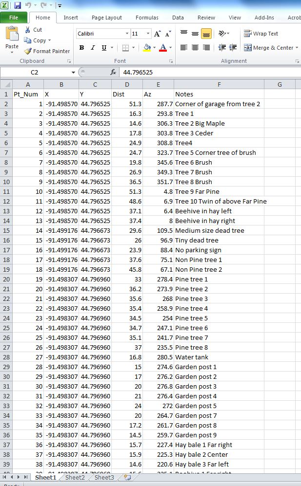
This spreadsheet only had 6 columns, instead of 7, because we only took 1 distance this reading this. They were titled the same as described above, except in a different order, and contained the same information.
Again, the spreadsheet was imported into our geodatabase, and the Bearing Distance to Line Tool was run. Again, the tool executed but the lines were in the middle of nowhere, the same place there were with the first survey. So, we again used the identify tool in ArcMap to get the lat/long of our 3 corners. We entered these numbers into our spreadsheet, imported it, and ran the tool. This time it worked (image 28).
Image 28: Lines created from our distance and azimuth recording using
the “Bearing Distance to Line” command

Next, we had to convert our data to points. Again, we did
this by using the “Feature Vertices to Points” command. The tool ran and
executed properly (image 29).
Image 29: Points created using the "Feature Vertices to Points” command

Results
Our first survey went well for the most part. All our
distances were on, but we had 3 azimuths that were wrong; this caused our lines
to go into the direction (image 30).
Image 30: Results of our first survey

Here you can see the azimuths are off. We think this
happened because we weren’t using the device properly. We realized we weren’t
holding the button down until a recording came onto the screen; we just hit the
button and released it.
The results for the second survey were ok, but could’ve been better (image 31).
Image 31: Results of our second survey

Because the area is so densely populated with trees, it was
hard to find the exact locations of where were taking our shots from on the
aerial image. Therefore, we don’t know how accurate our X and Y locations are.
We know either the first or second tree location is wrong because the lines on
the far left side should match up with one another. The image was also hard to
work from because it is out dated and doesn’t have any of the features, besides
the trees, that we were shooting at. Therefore it’s hard to tell exactly how
accurate we were. We also realized our azimuth and distance was off for our
garage corner shots. We aren’t sure if this is because the points we were
shooting at were small and the laser was recording something else, this still
confuses us.
The following images are shots of our survey results at different scales (images 32-35).
Image 32: Both surveys after completion with lines and points at a
larger scale


Image 33: Both surveys after completion with lines and points at a
smaller scale

Image 34: Both surveys after completion with only points at a larger
scale

Image 35: Both surveys after completion with only points at a smaller
scale

Discussion
There are still a few things that need to be cleared up with
this survey method and ArcMap. One of them is understanding why the azimuth is
sometimes in correct with the laser, and the distance for that matter. Is it
the operator of the laser? It seemed to work fine most of the time and other
times not so well. But, if the operator was doing it the same every time why
all of the sudden would something change to skew the readings? Another thing
that confused me with this lab was trying to understand why Google Earth and
GPS lat/long locations didn’t match up in ArcMap. They should always be the
same no matter where you are in the world or what tools you are using to get
them with. I don’t know if it had something to do with the projection of the
map or what. Overall, I feel as though this is a very powerful survey method, and
quite easy for that matter. Clearly having a survey station would be much less
time consuming and more accurate. However, if this technique needed to be
utilized in the field, it would provide very useful and accurate itself.
Conclusion
Overall, I learned that you cannot count on technology, and
you can never be too prepared. We should have taken the distance finder and
compass out with us both times. This would have saved time when the batteries
went dead on the laser. We also should’ve been routinely checking azimuth with
the compass, and distance with the distance finder, and compared that to our
laser results to make sure there we no crazy readings; which we got for both
surveys. I also learned the importance of lat/long accuracy and having a method
to get accurate readings. This is something I still need to look into more to
figure out, as I discussed under the discussion section. I also learned we
needed a better method for delineating our survey area. No features on the land
are ever going to line up perfectly for a survey plot. A measuring tape,
stakes, and ribbon all should’ve been used to measure out the area and section
it off from the rest. Last, but not least, like the other surveys I realized
how big of an impact time and weather can have on survey. If it’s cold and your
short on time your mind set might not be where it needs to be in order to
capture the best representation of the land as you might want. It was a chilly
day outside again. We both dressed warm but being cold outside always puts a
damper on things. And, like every other college student, we’re always in a
hurry to get to our next class, get our homework done, study, or get to work.
All factors that play into a survey not being as complete or accurate as you
would like.
No comments:
Post a Comment