This week’s field activity was a continuation of the last
three weeks field activities, which involved creating a navigational map,
learning to navigate using that map and a compass, and learning to navigate
using only a GPS unit. The purpose of this week’s field activity was to learn
how to navigate using a global positioning system (GPS) unit, with the ability
to rely on the maps we created. To do this each team was provided with the
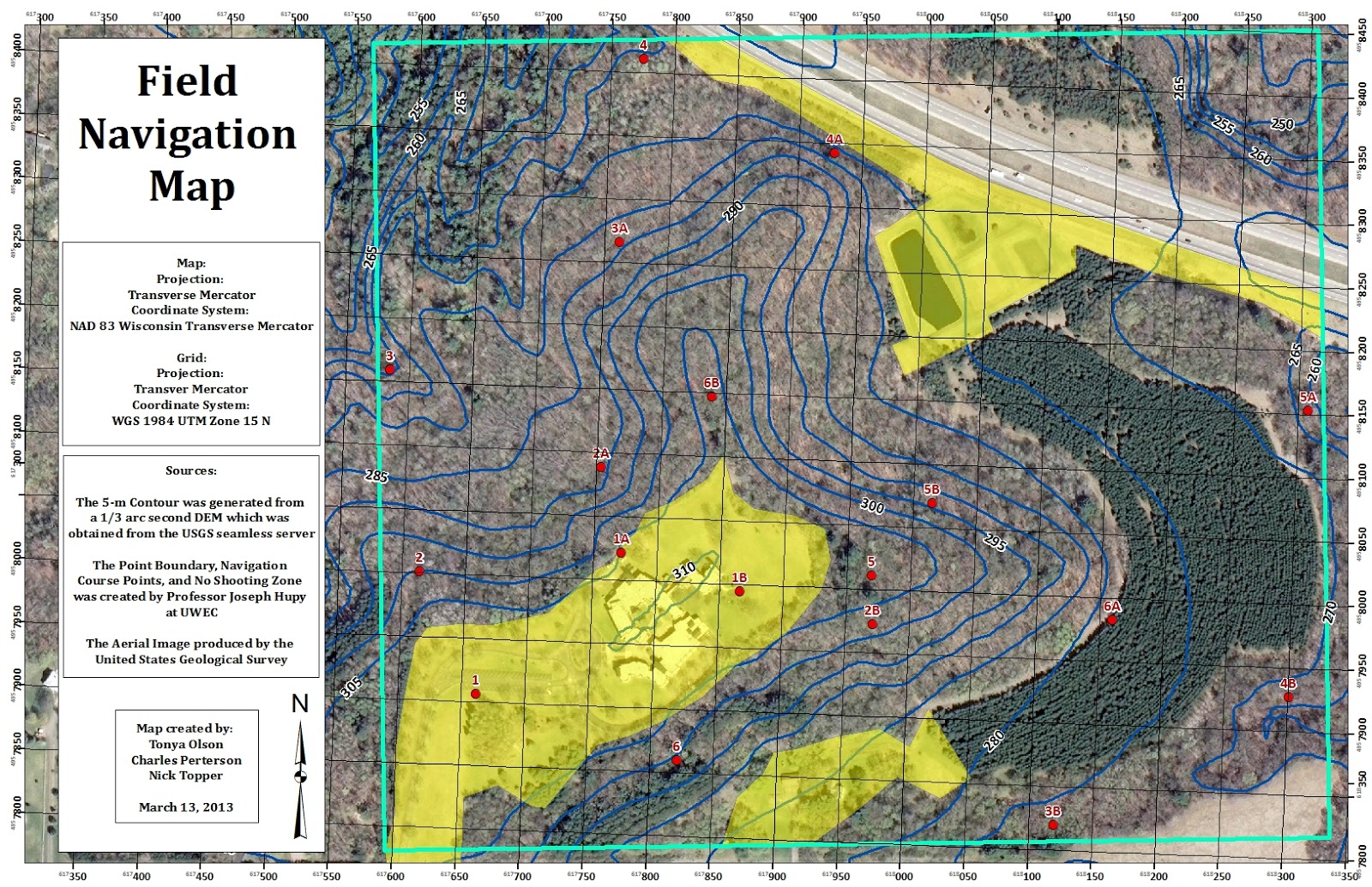
landscape terrain maps they created (images 1 and 2). Our professor also
provided each person with a sheet of paper that contained a series of points,
which coincided with the points on our maps, which contained their latitude and
longitude (lat/long) coordinate locations (image 3). Every person was also
provided with GPS unit (image 4).
Image 1: Navigational
map of landscape terrain created in a previous week’s lab
Image 2: Reference
side of the navigation map created in a previous week’s lab
Image 3: Sheet
provided to us by our professor with the point’s coordinate location
Image 4: GPS unit used
for navigation

The catch with this week’s activity is that paintballing was
incorporated into it. We had used all the methods in the previous week’s
activities, and updated our maps to better assist us in the field. Because of
this we were very familiar with the tools we had to navigate with, the pros and
cons of each of them, and the landscape we were traversing. The purpose of the
paintballing was to add a little fun into the mix, and also to encourage us to
use our skills wisely and efficiently. The area we navigated had a total of 15
points we were instructed to locate. This time we didn’t have a specific course
to navigate through; all six teams simply navigated the points as they felt was
most efficient. Navigating from point to point involved matching the lat/long
location on the sheet of paper to the lat/long on the GPS unit (image 5).
Latitude measures your location north and south, while longitude measures
location east and west. Because of this a compass provided in the GPS came in
very handy (image 6). Navigating also involved reading the terrain of the
landscape we were traversing using our map’s contour lines.
Image 5: Location of
lat/long coordinates on the GPS unit
Image 6: Compass on
GPS used for traversing from point to point
As mentioned in the last two week’s activities, as well as
Field Activity #4: Distance and Azimuth Survey, before one can use a compass
they need to check the magnetic declination of the place they are using it at.
Magnetic declination is the angle between compass north and true north. Compass
north is the direction the north end of a compass needle points, while true
north is the direction along the earth's surface towards the geographic North
Pole. Magnetic declination varies both from place to place and with time. In
Field Activity #4 we established that the magnetic declination of Eau Claire,
WI was 0ᵒ 59’ W. Since 0ᵒ is such a small declination no adjustments to the
compass is necessary.
Location
The area where the navigation took place was located on the
outskirts of Eau Claire, WI at a place called The Priory (image 7). This land
parcel is owned by the University of Wisconsin Eau Claire. This space is used
as the university day care center. Because of this restricted areas needed to
be added to our navigational maps. We needed to stay a safe distance away from
where the children utilize the area for safety reasons regarding them.
Image 7: Locational
map of the The Priory in Eau Claire, WI where the navigational activities take
place
Methods
Updating Our Maps
Before we could actually begin the navigation part of this
activity each group’s maps needed to be updated. This involved adding the course’s
navigation points and numbering them, and adding the no shooting zones feature
classes. We also needed to make corrections to our maps based on things that
could be improved upon to allow for more efficient navigating. Our group was
very happy with the first map we created so all we added was the labeled points
and the no shooting areas (images 8 and 9).
Image 8: Navigation
Map with the course’s navigation points labeled and the no shooting zones added
The red dots with a
number and letter above them represent the course’s navigation points and the
yellow zones represent the no shooting zones
Image 9: Reference Map
with the course’s navigation points labeled and the no shooting zones added
The red dots with a
number and letter above them represent the course’s navigation points and the
yellow zones represent the no shooting zones
Getting Ready For The Navigation
To begin this activity we had to haul all the equipment
(image 10), which included paintball guns, safety masks, and snow shoes, out to
The Priory. We then had to get all the equipment set up in an organized manner
(image 11 and 12). Getting the paintball
guns set up involved screwing all the pieces of the gun together and filling
the guns with paintballs (image 13).
Image 10: Truck used
to haul all the equipment out to The Priory
Image 11: Getting all
the paintball guns and safety glasses laid out in an organized manner
Image 12: Getting the
snow shoes out for everyone to take a pair
Image 13: Filling the
guns with paintballs
Each person then had to select a paintball gun, safety mask,
and pair of snow shoes (snow shoes were optional for whoever wanted to use
them) to use and get themselves prepared for the navigation (images 14 and 15).
Image 14: Getting snow
shoes on for whoever chose to wear them
Image 15: Set to
navigate with all the necessary equipment on
The Navigation
Before beginning the navigation each person needed to turn
on the track log on their GPS unit (image 16). Once the track log is turned on
the GPS unit begins tracking the route you walk. It is very important to turn
this on otherwise you will not end up with any data at the end of your
navigation to see how well you traversed from point to point using the lat/long
coordinates and your map.
Image 16: Location on
the GPS where the track log is turned on and off
To begin the navigation we all had to start from the same
starting point. At that time every team took a separate route of their choosing
to get to the first point they were navigating to. We were instructed we needed
to wait at least 5 minutes before any shooting began. This was intended for
safety reasons and to give each group time to separate from other groups and
actually focus on the navigation.
To locate the first point, our group agreed to traverse to,
we matched the GPS unit’s lat/long to the lat/long on the sheet of paper (image
17). We also used the map. By using the map we were able to match the elevation
we were starting at with the elevation of the first point we were navigating to
and use the 2-ft contour lines to determine how far down the hill we needed to
go. Using the map also useful because we were able to see which direction we
needed to go. By doing this we could
match the compass on the GPS unit with that direction. This was also an
efficient method because the lat/long and the compass are located on the same
screen on the GPS so you don’t have to switch between screens while navigating
(image 18).
Image 17: GPS unit
used to navigate from point to point by matching the lat/long to the sheet of
paper with lat/long coordinates for each point
Image 18: Lat/long
coordinates and compass located on same screen for more efficient tracking of
directional movement
Once a navigation point was reached (image 19) we used the
hole punch provided to punch the number point sheets that were provided to us
(images 20-22). We also took a way mark on our GPS unit’s.
Image 19: Point
marking the navigation courses
Image 20: Sheet
provided to us to punch with the hole punch once they were navigated to
Image 21: Sheet
provided to us to punch with the hole punch once they were navigated to
Image 22: Sheet
provided to us to punch with the hole punch once they were navigated to
We continued to navigate the course using this method until
class time was over. At this point we
headed by to the starting pint and turned our track logs off. It was important
to turn the track log off because otherwise anywhere you went after the
navigation activity was over would be recorded. This would make it extremely
difficult to know your course when the file was downloaded to the
computer.
Downloading The Data
Following the navigation activity we needed to get our track
logs and way points downloaded from our GPS units to a computer.
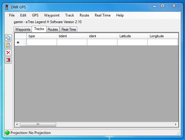
To do this I used a program called DNR GPS was that was
already installed on the computers (image 23).
Image 23: The DNR GPS
program used to download my track log points onto the computer
The following steps will lead you through the process that
was executed to get the data from my GPS unit onto the computer.
1. First,
the GPS unit needed to be connected to the computer with a USB port cord (image
24).
Image 24: GPS unit
connected to the computer with a USB port cord
2. Then, the “Track” tab was
selected (image 25).
Image 25 : “Track” tab selected
3. Next, the “Track” tab at the
top of the screen was selected and “Download” was chosen (image 26).
Image 26: “Download”
was chosen from the “Track” tab dropdown menu
4. Then,
the computer downloaded the track log data from the GPS unit (image 27).
Image 27: Computer
downloaded track log data from GPS unit
5. Next,
the data was saved into my personal class folder on the W drive as a point
shapefile (images 28 -30).
Image 28: “Save to”
then “File” is chosen from the “File” dropdown menu
Image 29: Navigate to
my class folder to save my data as an “ESRI Shapefile”
Image 30: Chose to
save my data as a “point” shapefile
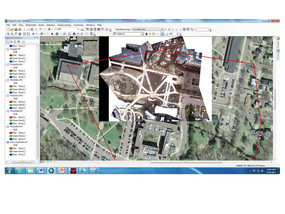
After the track log was downloaded into my class folder I
created a geodatabase, in my class folder, using ArcCatalog. Here, I imported
my shapefile as feature class. Next, I brought my track log into ArcMap (image
31).
Image 31: Track log
brought into ArcMap as a point shapefile
After checking the projection of my track log I saw that is
was in GCS_WGS_1984 (image 32). It was projected in this coordinate system
because that’s what the GPS unit I was using was set up as.
Image 32: Track log
downloaded in a GCS_WGS_1984 coordinate system
However, the professor instructed us to have our track logs
projected in UTM Nad 83. So, I projected my track log into NAD 1983 UTM Zone
15N (images 33 and 34). This is because Eau Claire, WI is located in UTM Zone
15 North.
Image 33: Using the
toolbox in ArcMap to project my track log feature class into the correct
projection
Image 34: NAD 1983 UTM
Zone 15N as the chosen projection for my track log
Finally, I was able to bring my track log into a new blank
map in ArcMap (image 35). By doing this, the data frame for the map was set to
this projection due to project on the fly.
Image 35: My track log
after the projection
After getting my track log data download I needed to get my
way point data downloaded. To do this I followed the same steps as outlined
above, except selected the appropriate “Waypoint/s” tabs instead (image 36).
Image 36: “Waypoint/s”
tabs to be selected to download way point data
Now I was able to create maps that depicted the navigation
routes for myself, my group, and all groups combined.
Results
Map 1 depicts my individual track log. It shows that overall
navigation from point to point was a little curvy. I didn’t walk in a straight
line from point to point; however some were better than others. When comparing
my final navigation, using both a GPS unit and a map, to my second navigation
(map 2) of using only a GPS unit you can similarities in the curviness of my
routes.
Map 1: My individual
track route and way points from the final navigation activity using a GPS unit
and a map
Map 2: My individual
track route from the second navigation activity using only a GPS unit
Map 3 illustrates my groups track logs. Here we can see that
overall we followed similar paths. When comparing it to map 4 we can see that this
was also the same in comparison to our second navigation. However, there are
certain areas in our routes that show times when we split up slightly from one
another. This is most vivid in the patch of pine trees in the southwestern
section of the map. This is due to our group coming in contact with another
group and having a paintball war with one another.
Map 3: My groups track
routes and way points in relation to one another’s from the final navigation
activity using a GPS unit and a map
Map 4: My groups track
routes and way points in relation to one another’s from the second navigation
activity using only a GPS unit
Map 5 shows the routes for all 6 groups. Team’s routes and way points are depicted
through color coding. For example the same color genre from light to dark.
Overall, we can see that teams typically followed similar paths. This is the
same when compared to map 6.
Map 5: All six groups
track routes and way points in relation to each other from the final navigation
activity using a GPS unit and a map
Map 6: All six groups
track routes and way points in relation to each other from the second
navigation activity using only a GPS unit
Discussion
Overall, we can see similar patterns in how teams routes
overlapped one another’s in most cases. Clearly map 5 shows very unstable
routes in comparison to map 6. This is because there was no preset path or
course to follow. In comparison to the previous weeks routes I didn’t think that
the curviness of the paths differed too much. In all, we found the using the
map was helpful and found that we rarely used our GPS units at all.
By taking way points on our GPS units we were able to
compare them to the course navigation points that were given to us. By
comparing how the two lined up in relation to one another we were able to see
how technology is not always perfect. Needless to say we didn’t get to all of
the points in the time we were for this activity. Fifteen points was a lot to try to get to in
the spread out area we were navigating in 2.5 hours we had to collect them all.
Conclusion
From this activity I learned several important aspects
involving navigational skills, keys to success for future navigation, and the
pros and cons of the tools involved. Throughout all the navigational activities
we’ve conducted this semester I’ve learned the importance of team work. At
first working on a team to some may just seems nice to have others around to
visit with and make the time more enjoyable. To others who like working alone
it may seem annoying and stressful. But what I’ve learned from all these
experiences is that working in a team provided us with efficiency and success.
Our team worked very well together and everyone brought different strengths to
the board. This proved very helpful for certain aspects. For example, one of
our team members had very long legs and was good at keeping pace counts in the
deep snow. Another team member was very good at tacking locations using the
lat/long on the compass.
I also learned that’s it’s very important to be familiar
with the gear you are using in the field before going out and trying to
accomplish an important task with it. For example, my protective face mask kept
fogging up on me. This was extremely annoying, inefficient, and unsafe. I had
to keep stopping to take off my mask and wipe the clear area off I looked through.
This slowed us down and was very unsafe for in the event there may have been
another group around who may have started shooting at us. I also found the snow
shoes to pose difficulty. Overall, I thought walking through the snow in them
was much easier. However, I kept stepping on the backs of my own snow shoes
with the opposite foot and kept falling down. This slowed us down, tired me
out, and I kept smacking my shins on branches laying down under the snow. They
were also hard to maneuver quickly in. When another team was present and you
were trying to get low, hide behind a tree to position yourself in a safe place
to shoot at them it was very difficult to do because they were so large and
clunky. Finally, I found that the gun got very heavy at by the middle of the
navigation. Again, this made me tired and slowed me down. Next time I would
choose to put a stack on my gun so I could carry it over my shoulders.
Finally, I learned the importance and pros and cons off all
the navigational tools were used. I found that I liked using the map the best.
However, I can’t say that the map alone is sufficient. For the last navigation
activity we were pretty familiar with the landscape, since we had already
navigated two courses in previous weeks. The area was also fairly small, not
small in the sense that it was too small for this activity, just in the sense
that we could determine our placement on the course in relation to the
interstate and the day care center building. This made the last navigation
easier than the first two because we could look at the map, determine our
position, and remember the terrain of the landscape we were looking for to get
to our next way point. Not only that, but the 2-ft contour lines made it very
easy to determine ridges, valleys and flat areas. This was especially helpful
in reading the landscape. I found that I liked the first method of azimuth and
pace count, with the map the best. I thought using azimuth with the compass
made the direction we needed to travel very straight forward, and the pace
count worked well for determining distance. However, I do think that without
having my team members for pace count that I would’ve done as good, or been as
happy with the method. Again, this plays into the fact of the high snow and me
having short legs. I think that pace count would be much easier when there is
no snow on the ground. I also like the azimuth and pace count method because
technology can always fail you. So if you started off using a GPS unit and the
batteries died you could always rely on your never failing compass and pace
count. Overall, I found the GPS unit to be difficult to use alone without a
map. The second time we used it with the map it didn’t come in as handy as the
first week because we were familiar with the landscape and had our map. I think
the GPS unit and map together would complement one another very well in an
unknown landscape.