Field Activity #10: Collecting Data and Creating a Database Using a Trimble Juno GPS Unit

Introduction

The purpose of this week’s field activity was to collect data at The Priory using a Trimble Juno GPS unit (image 1). This data will be the beginning to an ongoing database of what The Priory has to offer, in regards to recreation and sportsman’s activities, and to begin restoration of the grounds. Features of interest include: trails, benches, erosion points, notable views, large/notable trees, dead trees (with lots of woodpecker holes), human objects (garbage, dumps, fences, deer stands, etc.), bluebird houses, animal signs/track, etc. However, the goal of this week’s field activity wasn’t just to collect this type of data; we also learned how to develop a data collection procedure from the ground up.  To do this by each team decided on a feature/s to collect data for. It was each team member’s responsibility to develop a geodatabase that housed their GPS data, and apply appropriate attributes and domains to the database. After the data collection procedure we combined our group data together in the geodatabase.

Image 1: Trimble Juno GPS unit used to collect data

 

 

Study Area

The area where the data collection took place was located on the outskirts of Eau Claire, WI at a place called The Priory (image 2). This land parcel was recently purchase and is now owned by the University of Wisconsin Eau Claire. This space is now utilized as the university day care center. Within the parcel is a large wooded area containing many trails, benches, and wildlife.

Image 2: Locational map of the The Priory in Eau Claire, WI where the data collection activity took place

 

Methods

           Setting up the Folders

To begin this exercise we first had to create a geodatabase and deploy the geodatabase for ArcPad to the Juno GPS unit for the field data collection. To do this each team decided on a feature/s to collect data for. Our team chose to map and collect attributes for trails. First, we had to create a folder, within our class folder in the W drive, to store our information. We titled this “CheckInOut_username”.  For example, mine was title CheckInOut_olsonton. Then, we had to create a geodatabase within that folder titled Priory_username (Priory_olsonton). Next, had to create our feature class within the geodatabase. The feature class type is based on the type of data you are collecting. In our case, we chose trails; therefore our feature class type is a line feature class (image 3). We were instructed to set the projection for the feature classes to NAD_1983_HARN_Wisconsin_TM meters.

Image 3: Folder, geodatabase, and feature class locations for data collection within our class folder

 

Then, we had to set our domains for the data collection (image 4). Setting domains is important and useful as it allows for quicker data collection and eliminates the possibility for error; therefore, it contributes to more efficient and accurate data collection. Before domains can be set it’s important to know what type of information you’re going to be collecting in the field. In our case we chose to collect information of the condition, surface, and use of the trail. Within those groups we need to decide what categories we wanted available for selection. For condition we chose poor, fair, good, and excellent. For surface we chose dirt, gravel, paved, and other. For use we chose walking, four-wheeler, snowmobile, horseback, and other. It’s important to leave an “other” category in case you come along something unknown or unforeseen while you’re out collecting data. It leaves room for proper collection as you can write notes within the attribute table about these features. To create a domain, simply right click on the geodatabase, select properties, and select the Domain’s tab.

Image 4: Setting domains within a geodatabase

 

           Getting the Project Ready in ArcMap

Next, a project needs to be created to link your data to. First, I added the trails feature class I just created. I added this feature class first because it was in the desired projection. By adding this first I set my data frame projection to this due to ArcMap’s project on the fly feature. Next I added a raster image of Eau Claire and Zoomed into the priory. Then I added a boundary feature class of the location so I would be able to see the proximity in which were collecting data for (image 5).Finally I used the extract by mask tool to clip a large portion of the raster as it was unnecessary for the activity and raster files take up a lot of memory space.

Image 5: Project for data collection

 

Finally, you need to deploy your project to the GPS unit. By deploying the data, instead of just copying and pasting your folder, all the information within the geodatabase, such as the domains, are deployed with it.

To do this you first, you need to make sure the Arc Pad Data Manager is selected within the extensions (image 6). Do this by simply selecting customize at the top of the screen, and then extensions.

Image 6: Arc Pad Data Manager is selected within the extensions

 

Then you need to open the Arc Pad Data Manager within the toolbars (image 7). That again is located in the customize tab.

Image 7: Location of Arc Pad Data Manager within the toolbars selection

 

Next you need to select the Get Data For ArcPad button on the Arc Pad Data Manager toolbar (image 8).

Image 8: Location of the Get Data For ArcPad button on the Arc Pad Data Manager toolbar

 

Once the wizard opens you need to click Next on the welcome screen. Then click on the Action menu bar and choose Checkout all Geodatabase layers only (image 9). What that does is allows you to check out the data domain associated with the layers.

Image 9: Selecting Checkout all Geodatabase layers only on the Action menu bar

 

Next click on the raster image file and choose to Export as background JPEG2000 (image 10).

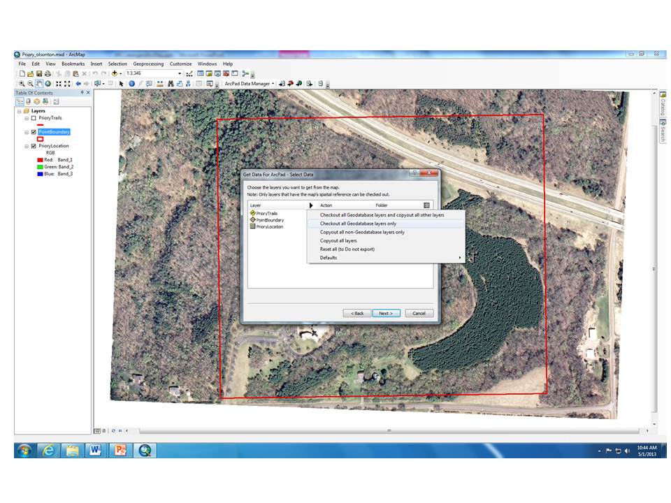
Image 10: Selecting to Export as background JPEG2000 for the raster file

 

On the next screen (picture options) simply hit next (unless you plan on taking pictures, then specify the location).

On the Select Output Options screen<!--[if !vml]--><!--[endif]--> under Specify a name for the folder that will be created to store the data: name it Priory_username (Priory_olsonton) (Image 11). Make sure you change the path where the file is to be stored (Image 11). Store the file in the CheckInOut folder created at the beginning of the exercise. Leave create an ArcPad map (.apm file) for the data checked, and make sure the .apm file is the same name as your project (Image 11). Finally, if you didn’t use extract by mask for the raster file while you were creating the project before deployment, make sure you select The current display extent from the drop down arrow (Image 11).

Image 11: Selection options in the Select Output Options screen

 

 

Once all your options and folders are selected and named properly hit next. On the final screen hit Finish. Now the Get Data For ArcPad wizard is complete.

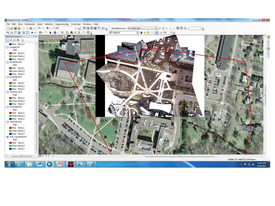
Next, we navigated to our class folders where we stored all our data. Here we were able to check and make sure everything saved properly. Here we can see the Priory_olsonton file we just went through the steps for creating (image 12). Here we also want to copy and repaste that folder. This is a backup file in case anything happens during deployment; this is will be a copy of the original file (image 12). This location also contains .apo files that are important for the check in and check out procedure (image 12). We can also see that our geodatabase and .mxd file are also located in this folder (image 12).

Image 12: Location of all the files created so far      

  

           Deploying the information onto the Juno GPS unit

First, you need to make sure the GPS unit is connected to the computer with a USB port cord (image 13).

Image 13: Juno GPS unit connected to the computer with a USB port cord

 

 

Then, we cut and pasted the folder we just created into the storage disk (SD) of the GPS unit.

A youtube video tutorial with step by step instructions for the outlined steps above can viewed at: http://www.youtube.com/watch?v=CzEAjP46020

           Collecting Data in the Field

Now we are ready to collect the data in the field. To do this we turned the GPS units on and selected ArcPad 10 on the menu screen (image 14).

Image14: Location of ArcPad 10 on menu screen

 

 

Then we selected Choose map to open (image 15).

Image 15: Selecting Choose map to open

 

Next, we located the .apm file we just created (image 16).

Image 16: Locating the .apm file just created

 

After it’s selected the map you just created will pop up (image 17).

Image 17: Map we be on screen once selected        

   

Once the satellite located our position we were ready to start at the beginning of our first trail. To map a trail and collect its data attributes we first selected the Quick Capture on the tool bar (Image 18). Then we selected the Line Capture Feature (image 18). Next we selected the Cancel Add GPS Vertex (image 18). This tool takes a vertex every time you selected it. As we walked along the trail we made sure to stop and hit Cancel Add GPS Vertex again every couple of feet in a curve or a corner to make sure we were capturing the true route of the trail. Once you are complete with a trail the vertices will create a line from the beginning of the trail to the end of it. If we hadn’t done that the trail would only show up as one straight line with no curves or corners. To finish a trail we hit Save Geometry Changes and then Proceed to Attribute Capture (image 18). Once Proceed to Attribute Capture is selected the attribute table automatically pops up and you can enter the attribute information. This where the domains we created earlier come in. Here is where the domains should be selectable from a drop down box. In our case, something went wrong with our initial set up and the domains weren’t applied to our trail feature class. So we had to enter our data in manually. This is where efficiency and accuracy come into place. With domains entering data would’ve been faster. Since each team member was only responsible for one category (condition, surface, or use) this wasn’t a big for us. Also with domains the possibility of entering data in incorrectly would’ve been avoided. This could be as simple as misspelling a word or having some words start with capital letters and others without capital letters. This would be an issue that would prove inefficient later while analyzing data. This could provide difficulty for later querying or mapping. Again because we didn’t have a lot of trails this won’t be a problem for us to quickly fix in ArcMap if needed. However, if this were a very large data set it could prove to be very time consuming and irritating.

Image 18: How to collect data using the Trimble Juno GPS unit in the field

 

We continued this same process for every trail we walked down.

          Checking the Data Back in from the Juno GPS unit 

Once data collection in the field is complete we got our data from the GPS unit onto a computer. To do this we hooked the GPS back up to a computer with a USB cord and navigate to the GPS unit’s SD location. From there we copied and pasted the folder back into our CheckInOut folder.

Next, we selected the Get Data From AcrPad (image 19) button on the Arc Pad Data Manager toolbar.

Image 19: Location of the Get Data From AcrPad button on the Arc Pad Data Manager toolbar

 

 

We then selected the green plus button on the Get Data From AcrPad screen and navigated to the folder we just checked in. After it’s selected it will occupy the Get Data From AcrPad screen. Then you select Check in (image 20).

Image 20: Location of buttons to retrieve data and check it in

 

Finally, your data will be in ArcMap (image 21).

Image 21: Data collected on Juno GPS unit is all in ArcMap

 

 

Results

Image 22 depicts the data I collected with my GPS unit. The attributes I collected included information regarding how the trails were utilized. Here we can see that the two categories include driving and walking trails. Since the trails weren’t labeled their use was determined in regards to the size and surface of the trail. If the trail was wide and paved I labeled it as driving and if the it was thin, dirt and through the woods I labeled it walking.

Image 22: Trail data I collected in regards to the type of use of the trail

 

 

Image 23 depicts the data collected with the GPS units by myself and my team members. The attributes collected for this map include the utilization of the trails, as explained above, the surface type and the overall condition the trail is in. If the trail was covered with an impervious surface then it was labeled paved and if it was a trail was not covered with an impervious surface and ran through the woods it was labeled dirt. When determining the condition the trail was in tree cover and dead branches laying over the trail were determining factors.

Image 23: Trail data collected in regards to the type of use, surface, and conditions of the trail

 

Overall, we can see that the majority of the trails are dirt. We can also see that the majority of the trails are in good or ok conditions. Finally, the use of the trails contains a fairly even distribution in regards to the type of the use.

Conclusion

Overall, I thought this was a very fun project. I think the idea of being able to create, not only a new map but a database that contains useful information about a place is very powerful. I think the Trimble Juno GPS units are very effective tools. It would be very cool to see a map of the all the data that was collected by all the groups mapped together.

One thing that became very apparent when creating the maps was the fact that we didn’t use the domains that we created before deploying our projects to our GPS units. As discussed earlier, for whatever reason, our domains didn’t transfer with our projects onto our GPS units. This didn’t really provide a problem in the field for our data collection due to there being only a few trails. However, had there been a ton of trails or had we had been collecting a lot of data for a very tedious project this would’ve proved very inefficient. While making the maps I did come across two separate instances where I had to fix the attribute table in order for everything to map correctly. For example “ok” in the conditions column was spelled with both letters lowercase and other times with the “O” as a capital letter. When attempting to map conditions in this way they show up as two separate attributes instead of just one. However, like I said before, this was an easy fix since there were only a few maps. Had there been a huge database with this issue fixing it would’ve taken much longer and would’ve been very irritating.

 

 

 

 

 

 

 

Field Activity #9: Georeferencing and Mosaicking

Introduction

The purpose of this week’s field post is to discuss the process involved in georeferencing and mosaicking aerial imagery, in Arc Map, that was obtained through balloon mapping (balloon mapping is discussed in further detail in the blog post titled “Field Activity #3: Construction of Field Mapping Equipment”).

Methods

          Importance of Good Quality Images

Before the georeferencing process can begin it’s necessary to look through images that were obtained to find ones that will work well. This includes finding images where the shot is perpendicular to the ground (images 1 and 2), images that can overlap one another, and images that are not blurry (image 3). These factors are important for several reasons including, shots that are perpendicular to the ground will have less distortion in the center of the picture compared to the edges.  Therefore when you overlap several pictures together they will depict a realistic view of the ground.  When the camera is not parallel to the ground the images will be very distorted, therefore the do not depict a realistic view of the ground. Images that are fuzzy or not clear will also not depict a realistic view of the ground.

Image 1: Camera shot that is perpendicular to the ground

Images that are perpendicular to the ground will have less distortion in the center of the picture so they will work the best for depicting a realistic view of the ground

Image 2: Camera shot is not perpendicular to the ground

When the camera is not perpendicular to the ground the images will be very distorted, therefore not depicting a realistic view of the ground

Image 3: fuzzy or not clear image

Images that are fuzz, or not clear will also not depict a realistic view of the ground

Images 4 - 13 are the images I chose to use.

Image 4: Image chose for georeferencing in my first mosaic

Image 5: Image chose for georeferencing in my first mosaic

Image 6: Image chose for georeferencing in my first mosaic

Image 7: Image chose for georeferencing in my first mosaic

Image 8: Image chose for georeferencing in my first mosaic

Image 9: Image chose for georeferencing in my second mosaic

Image 10: Image chose for georeferencing in my second mosaic

Image 11: Image chose for georeferencing in my second mosaic

Image 12: Image chose for georeferencing in my second mosaic

Image 13: Image chose for georeferencing in my second mosaic

          Georeferencing

To begin the georeferencing portion of the activity I first started a new project in Arc Map. I then opened the georeferencing tool bar (image 14). Next, I brought in the control points feature class. This feature class was created by 3 students using 3 different types of GPS units. This was done to provide ground control points to georeference too. I brought this feature class in first because it set the data frame to UTM 15N through Arc Map’s Project on the Fly feature. Next, I brought in the aerial image of the campus location that was provided for us by our professor. Then I brought in group 5’s feature class. This is a polygon feature class that was created by 2 of the students in the class who took the initiative to divide campus into 6 areas so each group could focus in one main area. This allowed for better use of time and accuracy as the area we all had to cover was much smaller and people weren’t all mapping the same area or leaving an area out. Finally, I brought in the first image I wanted to georeference.

Image 14: Location of the “Georeferencing” tool bar

Steps to georeferencing:

1) To begin georeferencing I zoomed into the area I would be georeferencing to on the aerial photo, with in group 5’s designated area.

2) Then, I made sure the image I was georeferencing was selected in the georeferencing tool bar drop down box (image 15).

Image 15: Selecting the correct image to be georeferenced in the georeferencing tool bar drop down box

3) Next, I selected “Fit to Display” from the georeferencing drop down menu (image 16). This fits the image you want to georeference into the display extent you zoomed into (image 17).

Image 16: Selecting “Fit to Display” from the georeferencing drop down menu

Image 17: Image fit within the display extent zoomed into

4) Then, I was able to use the “Rotate”, “Shift”, and “Scale” tools (image 18) to get my image to the rotation, spot, and size, that best suited the aerial image (image 19).

Image 18: Georeferencing tools used to rotate, shift, and scale the image being georeferenced

Image 19: Image rotated, sized, and moved to best fit the area

5) Next, I need to determine where my control points should be placed. By highlighting the ground point and viewing what feature it’s depicting I am able to determine where the ground point is located on the image being georeferenced (image 20). In this case the ground point is depicting a light pole. By looking at the image I am able to see that there is only one light pole nearby. Because of this I am able to determine that these two features should be located in the same spot. Therefore I will add a control point from the base of the light pole on the image to the control point.  

Image 20: Determining placement of control points

6) Then, I selected “Add Control Points” from the georeferencing tool bar (image 21). This allows me to add control points from the image I’m georeferencing to the aerial photo (image 22). At least 10 control points should be used for all photos being georeferenced to allow for accurate placement of the photo.

Image 21: “Add Control Points” selected from the georeferencing tool bar

Image 22: Adding control points from the image I’m georeferencing to the aerial photo

Finally, I was able to select “Update Georeferencing” from the georeferencing drop down menu (image 23). This saves the photo in place in relation to the control points you add.

Image 23: “Update Georeferencing” selected from the georeferencing drop down menu

This process was repeated for every image georeferenced. After all the images were georeferenced I exported them as raster files (image 24). This I needed to save the spatial reference of the image before mosaicking can be done.

Image 24: Exporting the georeferenced as a raster file

Here you need to select to have spatial reference saved the same as the data frame, selected your output location, name the file, and save it as a TIFF.

Image 25 depicts my images after they were all georeferenced and exported.

Image 25: Images after being georeferenced and exported

Finally, I was able to mosaic my images together. To do this I selected “Mosaic to New Raster” in the tool box (image 26).

Image26: Location of “Mosaic to New Raster” tool in the tool box

To run this tool properly it’s important to add all the images you want to mosaic, define your output location, name your output image and specify which type of file you would like to save it as. You can choose to save them as either a .tif or .jpg files. You must also specify the number of bands, which should be 3, and the mosaic operator. The mosaic operator runs the images in the order you specify. For example, I chose first meaning the first image I have listed (image 11 in image 27) will be the top image of my mosaic (image 27).

Image 27: How to fill out the “Mosaic to New Raster” tool

Image 28 shows my mosaic after this whole process was complete.

Image 28: Final completed mosaic

To observe how well my mosaic lined up with the aerial photo I used the “Swipe” tool located in the “Effects” tool bar (images 29 and 30).

Image 29: Location of “Effects” tool bar

Image 30: Location of “Swipe” tool in “Effects” tool bar

Overall we can see that my mosaic matches pretty well, but certainly isn’t perfect (image 31).

Image 31: Using the swipe tool to check my mosaic in relation to the aerial photo

Discussion

Overall, georeferencing is easy and difficult at the same time. The method itself is easy to perform, although it can be quite time consuming. However, making the overall mosaic line up perfectly was very difficult. As we discussed earlier, the center of an image taken when the shot is perpendicular to the ground is less distorted than the outside of the image. This is because of the angle at which the shot is taken. Because of this, it’s safe to use about the center 60% the image for georeferencing. However, the UWEC campus, which we’re creating an aerial map of, is under construction. Therefore, there are no updated aerial maps available as the reference, or ground point, map. Because of this our group had to rely solely on the ground points taken by the GPS units to georeference our data because our area to mosaic was located where a building has been removed and sidewalks have been added. This made georeferencing our data extremely difficult. The majority of the time we had no clue if our georeference lined up well or not because there were no sidewalks in the old aerial photo to compare them to. I did make a new map of the area of campus located over Phillips Hall (image 32) just to test my strategy. With this map I used georeferenced my control points to ground points, and tops of buildings. I also used the outside of my images, and a larger amount of control points; sometimes up to 30 or 40 control points on one image. Overall, this image turned out ok, but I know it was really distorted due to my manipulation of the photos.  

Image 32: Second attempt at a mosaic using sloppier methods to compare to my original mosaic

Conclusion

With this activity I learned the importance of very accurate ground control points. Without accurate ground control points it’s nearly impossible to create an aerial map that depict the landscape below. I also learned that no matter how much you want to make something turn out good it’s never a good idea to manipulate things to work for your benefit. Had I used the second map I created it may have had significant implications down the road to someone who may have tried to use it for something important. For example, if someone planned on using it for measurement the measurement would probably be off by a lot for them.

I also learned that it is important to have your camera on the right setting for the intended purpose of your field activity. We accidentally had our camera set on “normal” mode instead of “scenery”. This resulted in the camera being out of focus a lot of the time. This isn’t good because it’s important to have as many good pictures as possible to create a realistic aerial map.