Field Activity #7: Navigation with a GPS Unit

Introduction

This week’s field activity was a continuation of the last two weeks field activities, which involved creating a navigational map and learning to navigate using that map and a compass. The purpose of this week’s field activity was to learn how to navigate using a global positioning system (GPS) unit, without the assistance of a map. To do this our professor provided each person with a sheet of paper that contained a series of points with their latitude and longitude (lat/long) coordinate locations (image 1). Every person was also provided with GPS unit (image 2).

Image 1: Sheet provided to us by our professor with the point’s lat/long coordinate location

 

Image 2: GPS unit used for navigation

 

The area which we navigated had to total of three courses that were all overlapping one another. Two teams traversed on one course at a time with one team navigating from point 1 to point 6, while the other team traversed backwards from point 1 back around to point 2. Navigating from point to point involved matching the lat/long location on the sheet of paper to the lat/long on the GPS unit (image 3). Latitude measures your location north and south, while longitude measures location east and west. Because of this a compass provided in the GPS came in very handy (image 4).

Image 3: Location of lat/long coordinates on the GPS unit

 

Image 4: Compass on GPS used for traversing from point to point

 

 

As mentioned in last week’s activity, as well as Field Activity #4: Distance and Azimuth Survey, before one can use a compass they need to check the magnetic declination of the place they are using it at. Magnetic declination is the angle between compass north and true north. Compass north is the direction the north end of a compass needle points, while true north is the direction along the earth's surface towards the geographic North Pole. Magnetic declination varies both from place to place and with time. In Field Activity #4 we established that the magnetic declination of Eau Claire, WI was 0ᵒ 59’ W. Since 0ᵒ is such a small declination no adjustments to the compass is necessary.

Methods

To begin this activity we first had to locate our starting point. As mentioned above, we did this by matching the lat/long of the GPS unit to the lat/long point 1 provided on the sheet of paper (image 5).

Image 5: GPS unit used to navigate from point to point by matching the lat/long to the sheet of paper with lat/long coordinates for each point

 

Once we reached our starting point we turned our track log on (image 6). Once the track log is turned on the GPS unit begins tracking the route you walk. It is very important to turn this on otherwise you will not end up with any data at the end of your navigation to see how well you traversed from point to point using lat/long coordinates.

Image 6: Location on the GPS where the track log is turned on and off

 

 

After locating our starting position we navigated to the other 5 points (image 7) on our course by matching the GPS unit’s lat/long to the lat/long on the sheet of paper for the next point we were traversing to.

Image 7: Point markings the navigation courses

 

 

To accomplish this as efficiently as possible our team created a system. The system involved one person paying attention to the latitude, one person paying attention the longitude, and the third person kind of paying attention to both. We did this because it’s hard to focus on two separate numbers at the same time. This way it was less confusing and frustrating. If one person was watching their number and realized the value was getting higher instead of lower, or vice versa, then they could let the other team members know and the direction of movement could be corrected.

We also used the compass, located on the same screen as the lat/long coordinates (image 8), to help us get a better idea of which direction we needed to be walking. As mentioned earlier, this is because latitude measures your location north and south, while longitude measures location east and west.

Image 8: Lat/long coordinates and compass located on same screen for more efficient tracking of directional movement

 

 

Once the final point was navigated to the track log was turned off. It was important to turn the track log off because otherwise anywhere you went after the navigation activity was over would be recorded. This would make it extremely difficult to know your course when the file was downloaded to the computer. 

After the navigation was done every person downloaded their data from their GPS unit onto a computer as shapefiles. To do this I used a program called DNR GPS was that was already installed on the computers (image 9).

Image 9: The DNR GPS program used to download my track log points onto the computer

 

 

The following steps will lead you through the process that was executed to get the data from my GPS unit onto the computer.

1. First, the GPS unit needed to be connected to the computer with a USB port cord (image 10).

Image 10: GPS unit connected to the computer with a USB port cord

 

2. Then, the “Tracks” tab was selected (image 11).

 Image11 : “Tracks” tab selected

 

 

 3. Next, the “GPS” tab at the top of the screen was selected and “Connect to Default GPS” was chosen (image 12).

Image 12: “Connect to Default GPS” was chosen from the “GPS” dropdown menu

 

4. Then, the computer located the GPS unit that was connected to it (image 13).

 Image 13: Computer located the GPS unit that was connected to it

 

 

 5. Next, the “Track” tab at the top of the screen was selected and “Download” was chosen (image 14).

Image 14: “Download” was chosen from the “Track” tab dropdown menu

 

6. Then, the computer downloaded the track log data from the GPS unit (image 15).

Image 15: Computer downloaded track log data from GPS unit

 

7. Next, the data was saved into my personal class folder on the W drive as a point shapefile (images 16 -18).

Image 16: “Save to” then “File” is chosen from the “File” dropdown menu

 

Image 17: Navigate to my class folder to save my data as an “ESRI Shapefile”

 

 

Image 18: Chose to save my data as a “point” shapefile

 

 

After the track log was downloaded into my class folder I created a geodatabase, in my class folder, using ArcCatalog. Here, I imported my shapefile as feature class. Next, I brought my track log into ArcMap (image 19).

Image 19: Track log brought into ArcMap as a point shapefile

 
 

After checking the projection of my track log I saw that is was in GCS_WGS_1984 (image 20). It was projected in this coordinate system because that’s what the GPS unit I was using was set up as.

Image 20: Track log downloaded in a GCS_WGS_1984 coordinate system

 

 

However, the professor instructed us to have our track logs projected in UTM Nad 83. So, I projected my track log into NAD 1983 UTM Zone 15N (images 21 and 22). This is because Eau Claire, WI is located in UTM Zone 15 North.

Image 21: Using the toolbox in ArcMap to project my track log feature class into the correct projection

 

Image 22: NAD 1983 UTM Zone 15N as the chosen projection for my track log


 

 

Finally, I was able to bring my track log into a new blank map in ArcMap (image 23). By doing this, the data frame for the map was set to this projection due to project on the fly.

Image 23: My track log after the projection

 

Now I was able to create maps that depicted the navigation routes for myself, my group, and all groups combined.

Results

Map 1 depicts my individual track log. It shows that overall navigation from point to point was a little curvy. I certainly didn’t walk in a straight line from point to point.

Map 1: My individual track route

 

Map 2 illustrates my groups track logs. Here we can see that overall we followed similar paths. However, there are certain areas in our routes that show times when we split up slightly from one another.

Map 2: My groups track routes in relation to one another’s

 

Map 3 shows the routes for all 6 groups on all 3 courses.  Colors yellow, orange, and red depict one team, while colors purple, blue, and green depict the other team who are both navigating on the same course. If you refer to course 1, the course my group traversed, you can see the difference between the two groups’ routes that navigated the course.

Map 3: All six groups track routes in relation to each other

 

Discussion

In short, after reviewing that results of all the maps we can see that navigation from point to point wasn’t perfect form anyone, or any group. We can also see in every course both teams traversing the course took different routes. This goes to show that navigating using a GPS unit probably isn’t the most effective and efficient navigational technique. It would be interesting to see how the results would differ if a map depicting the landscape was involved in the process.   

Conclusion

Overall, I found this form of navigation to be much harder than using a compass and pace count. I found that a map would’ve been much more helpful with this exercise than having with the compass and pace count exercise. Having a map that depicted the landscape terrain would’ve assisted the group in knowing if the point being navigated to was on top of a ridge, or in a valley. This would’ve been helpful because it had just snowed a lot that day and throughout the prior weekend. This made traversing the landscape very difficult and tiring.

I also found that it would’ve been helpful to have had a plastic baggie to put the piece of paper in with the point’s locational data. This is because the water from the snow made the paper difficult to read (image 24).

Image 24: Paper with point locational information was hard to read due to it getting wet from the snow

 

 

I found that towards the end of the navigation I was asking my team members what the numbers were to make sure I was reading them correctly. If I would have been reading them wrong we could’ve ended up walking in the wrong direction. That would have really stunk!

Like the previous activity we found that it was important to keep an eye on the lat/long onour GPS units. This is because the courses intersected one another, so at times you would come to a point on your course that wasn’t your intended target. Being that this navigation exercise was more difficult than the last one, seeing a point on your course made it easy to be lured to it without thinking about whether it was yours or another team’s point.  We actually made this mistake and traveled out of our navigation route to get to a point we thought was ours. When we got to it there was another team there. After debating whose it was we realized we were wrong. This goes to show the importance of paying attention and following your coordinates. It also shows how weather conditions can influence how you think and work. Like I stated earlier there was a lot of snow and traversing the hilly landscape with the difficult navigation technique all led to us navigating poorly towards the end when we were tired.

Field Activity #6: Navigation with a Map and Compass

Introduction

This week’s field activity was a continuation from last week’s activity of creating a navigational map (images 1 and 2). The purpose of this week’s activity was to learn how to navigate using a map and compass. To do this, our professor provided us a series of points to plot on our map (image 3).

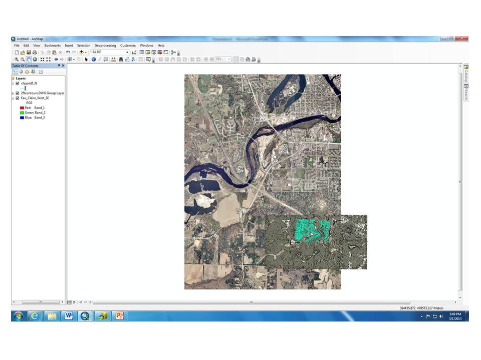
Image 1: Navigational map of landscape terrain created in previous week’s lab

 

Image 2: Reference side of the navigation map created in previous week’s lab

Image 3: Sheet provided to us by our professor with the points coordinate location

Then we had to establish a distance and azimuth from point to point in the direction we would be navigating. We established our azimuth using a compass. Azimuth is the angular distance along the horizon to the location of the object. It is measured from north towards the east along the horizon (image 4).

Image 4: How azimuth is determined

 

http://astrosun2.astro.cornell.edu/academics/courses/astro201/alt_az.htm

 

As mentioned in Field Activity #4: Distance and Azimuth Survey, before one can use a compass they need to check the magnetic declination of the place they are using it at. Magnetic declination is the angle between compass north and true north. Compass north is the direction the north end of a compass needle points, while true north is the direction along the earth's surface towards the geographic North Pole. Magnetic declination varies both from place to place and with time. In Field Activity #4 we established that the magnetic declination of Eau Claire, WI was 0ᵒ 59’ W. Since 0ᵒ is such a small declination no adjustments to the compass is necessary.

To establish our distance on the map we used the 50x50 meter grid. In the field we used the 100 meter pace count we establish the previous week.

After all of this was established we headed outside to one of the three established courses to locate our waypoints. Our team traversed course 3.

Methods

To begin this activity we plotted the points (image 5) provided to us by our professor, which correlated with the course our team would be traversing. We plotted our points using the UTM X and Y coordinates (image 6). We used these points because our map’s coordinate grid was established in a UTM projection.  

Image 5: Plotting our points

 

Image 6: Sheet provided for us by our professor with UTM X and Y locations of our waypoints

 

 

After plotting our points individually our team went through and compared out points to one another to make sure we had them plotted correctly.

Next, we had to establish a distance and azimuth from one point to another. Since there was a total of 6 teams and only 3 courses, 2 teams had to traverse the same course at the same time. So, one team worked from point 1 to point 6, and the other team worked backward from point 1 back to point 2. Our team worked backwards, so we went from point 1 to 6, then 5, 4, 3, 2 then back to 1 to finish. We established our azimuth using a compass (image 7).

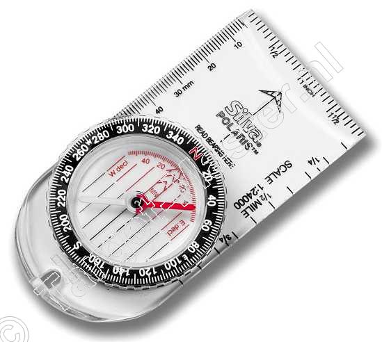
Image 7: Compass used to establish azimuth

 

http://www.target-master.nl/images/Silva%20Polaris%20177.JPG

1. First, I drew a line from point to point in the order we were going to be traveling.

2. Next, I laid my compass on my map with the center of the turnable housing unit (screw that holds needle in place) over the point I was starting at. For example, if I was working from point 1 to point 6, I laid it over point 1.

3. Then, I made sure north, on the turnable housing unit, was in the direction of north on my map (image 8).

Image 8: Turnable housing unit’s north in same direction as north on map

 

4. Next, I made sure the heading arrow was lined up with the line I drew from point 1 to point 6

5. Then, I read the number that correlated with the heading arrow; which is the azimuth; and wrote it on my map next to the line connecting the 2 points.

6. Lastly, all the team members compared their azimuth to each other’s to make sure we were all within a small range from one another (about 7◦ or less).

Next, we had to establish our distance from one point to the other in the order we were traversing. To do this we used the back side of the sheet of paper that had our point locations on it, and the ruler on the compass.

1. First, we lined the sheet of paper next to the grid on the map and made tick marks on it at every 50 meter increment.

2. Then, we labeled the tick marks with the corresponding distance from the map’s grid.

3. Next, we laid the paper on the map with a distance of 0 at the point we starting at to the point we were traversing to (image 9). For example, if we were measuring distance from point 1 to point 6 we place 0 at point 1 and measure the distance to point 6.

Image 9: Measuring distance from point we were traversing from to the point we were traversing to using a piece of paper with 50 meter increments measured  on it

 

4. If the point laid in a position where a 50 meter increment reading wasn’t accurate enough we used the ruler on the compass to get a more accurate reading.

5. Again, we compared our distances to one another to make sure we were all in an appropriate measurement from each other.

Once all distances and azimuths were established we created a chart that corresponded the distance and azimuth to appropriate point (image 10).

Image 10: Chart containing distance and azimuth with corresponding point

 

The last thing we did before going outside was poke a hole through the map from the navigation side to the reference side at each point (Image 11). We did this in so that if we needed to use the reference side of the map in the field we would know exactly where it was, without having to flip the map over several times. This would allow us to be more accurate and save time in the field if the reference side of the map was needed.

Image 11: Poking holes through the map from the navigation side to the reference side at each point

 

Finally, we were ready to go outside and execute the physical part of the navigation activity. For this we only took one of the 3 maps. This was because it is easier to have less to worry about and carry when hiking in the field.

To start, we shown where to start for the particular course we were navigating. For course 3 a tree was the starting point (image 12), also known as point 1.

Image 12: Starting point for course 1, also point 1 for that course

 

 

To get from point 1 to point 6 we referred to the distance and azimuth chart, we created for our course, and read the distance and azimuth for point 1 to point 6. Using the compass in the field for azimuth differed slightly from how we used it inside to establish azimuth on our maps.

1. First, we made sure the red N for north on the compass’s turnable housing unit was lined up the heading north arrow (image 13)

Image 13: North indicator on the turnable housing unit lined up the heading north arrow

 

2. Then, we held the compass with both hands on the beveled end of the base plate with the heading north arrow pointed directly perpendicular from our bodies. While doing this it is important to hold is slightly away from your body and also not close to any metal (i.e. rings on your fingers, button on your coat, etc.). This is because metal off-sets the compass needle slightly.

3. Next, we turned our entire bodies with the compass until we got the needle lined up directly with the red arrow inside the turnable housing unit (image 14).

Image 14: Needle lined up directly with the red arrow inside the turnable housing unit

 

 

4. Then, we found to the azimuth number on the turnable housing unit that corresponded with the azimuth on our chart and found a land marker in that vicinity to walk towards.

After the direction (azimuth) we needed to go was established we were ready to walk. This is where the pace count from last week came into play. Knowing how many paces we took in 100 meters made it easy to pace out since the distance we measured on our maps, using the grid, was in 50 meter increments. Being accurate with our pace counts was very important because we had 3 courses that were all overlapping one another. It was important to know how far you were so you didn’t see a point marker that intersected the marker you were going from to the marker you were going to and automatically assume it was the point you were looking for. If this happened, the next azimuth would be inaccurate with the direction you needed to go to get to your next point; and you would basically be lost for the rest of the navigation.

1. To be accurate with our pace counts we had one person walk first and stop when they got to 100 meters (image 15 and 16).

Image 15: First person walking 100 meters

 

Image 16: First person at their 100 meter pace count

 

 

2. Next, another group member walked and see how far their 100 meter pace compared to the first person.

3. If the two were accurate with one another one of the two would continue to walk.

4. The third person stayed back at the point we started from to make sure the two pacers stayed in line with the direction they were supposed to be heading.

5. After one of the walkers continued to walk a second increment the last person (the direction monitor) would walk to the pacer who stayed at the 100 meter mark.

6. We continued this trend until the marker was spotted (image 17 and 18)

Image 17: Looking for the marker upon approach

 

 

Image 18: Markers that marked the point we were navigating to

 

7. Finally, we punched a hole in our navigation sheet (image 19), with the provided hole puncher at the marker, to show that we had found our point.

Image 19: Holes punched in navigation sheet to show we had found our point

 

We continued this method until all 6 points were found.

Discussion

Overall, we found that our distances and azimuths were very accurate. We found that we barely needed to use our map at all. The one time we did use our map we found it very helpful because we thought we were a little off on our azimuth. This happened because it is hard to walk in a straight line when walking up and down steep ridges with trees and brush in your way. When you have to walk around things such as these it’s difficult to get back on the right path, while still maintaining accurate pace counts. Our map designed for the situation proved very appropriate for depicting the terrain of the landscape. We were easily able to locate, from both sets of contour lines, the top of the ridge we were standing on. From this we were able to see we needed to head more to the left or more to the right while walking down from the ridge to get to the point we were navigating to. We also found that we never needed to refer to the reference side of the map, which had the aerial photo on it, to try to figure out where we were.

From this we learned that generally, we were all pretty accurate with one another’s pace counts. Again, this was much easier on flat ground where trees and brush were minimal. One thing I learned is that you need to be consciences of your pace lengths when walking through snow and brush. Typically, I find that I’m a fast walker and walk take longer strides than most people my height. However, in these snowy, brushy, and hilly conditions I found that my strides were much smaller. I almost needed to count 2 paces as 1 at some points.

Conclusion

I can definitely say that I learned a lot from this activity. I am very happy that I had the opportunity to learn these skills. I definitely think that having us create our own maps made us much more aware of the importance of appropriate map styles for certain activities. I don’t think there is anything I would change about my map. The thing I found most useful about the map was the 2 foot and 5 meter contour lines. The 2 foot contour lines depicted the terrain very well. The 5 meter contour lines came in very handy because those were labeled with their elevation, so we were able to compare them to the 2 foot contours to know if the 2 foot contours were depicting a valley or ridge feature of the landscape.  Having the 2 foot contours labeled with their elevation would’ve made the map way too busy and confusing. From this, I also learned the importance of having accurate and detailed data for a map. I don’t think the 5 meter contours alone would’ve been as good at depicting the landscape terrain.

Last but not least, we can’t end this discussion without talking about how important it is to come prepared for the weather. All of the other outdoor field activities we’ve done this semester haven’t involved too much movement; more just standing around. So I dressed really, really warm knowing we would be knee deep in snow for parts of the day. What I found is that I dressed way to warm for the type of terrain we were traversing. I got hot immediately and needed to start unlayering. Although I was much more comfortable after taking off one my sweatshirts, I found it very annoying having to carry it the whole time (image 20). It was also difficult because it kept getting caught on brush and twigs.

Image 20: Carrying a sweatshirt through the entire course was very annoying and difficult

 

Field Activity #5: Development of Field Navigation Map

Introduction

The purpose of this activity was to create a navigation map that will be used for the following field activity. That activity will involve manually plotting waypoints and their associated coordinates that will be provided for us by the professor. To create this map several data sets were provided for us. From the given selection we were to create a map that would provide us with the ability to know the terrain we are traversing; as well as being able to plot the points within reasonable accuracy. This map also needed to include some type of coordinate system that would be appropriate for conducting a survey at a large geographic scale at the local level.

Methods

To begin, the first thing we did a class was go outside and establish our pace count. A pace count provides you with ability to know how many steps you take within a given distance. We did this because this will be our method for measuring the distance we travel during our survey for the following week. To do this we used a distance finder and established a distance of 100 meters. Then, the class walked to the distance 2 to 4 times to get an average consistency. My pace count was about 68-70 steps within the 100 meter distance.

Next, we went inside and started on to create our maps. Data set provided to us by the professor included color and black and white aerial images, a digital elevation model (DEM), a 2-foot contour line map, a 5-foot contour line map, a clipping boundary, and a point boundary. It was our choice for what which data sets we chose to utilize. We were given the guidance of being told that some of the best maps for this type of project are simple ones. Having a map that is “too busy” can impede on the navigation. We were also told we could make a two-sided map for reference purposes.

With that, I chose to use both the 2 and 5-foot contour data sets (images 1 and 2), the point boundary data set (image 3), and a 50x50 meter grid (image 4)for the main navigation map that will be used to plot the points. The 2-foot contour file was generated during a UWEC survey and the 5-foot contour file was generated from a 1/3 arc second DEM that was obtained from the United States Geological Survey (USGS) seamless server. I chose both the contours because together they create a very precise, yet simple, vision of the landscape terrain. The point boundary data was created for us by our professor. I used to the point boundary data set for reference of the specific area the points will be located within. Finally, the 50x50 meter grid is a feature that is created in Arc Map.  I chose a 50x50 meter dimension because I felt it was detailed enough for the terrain, and because I didn’t want the grid to be “too busy” and distracting. This size also works well because our pace count was based on 100 meters so I would be able to cut my pace count in half, to about 34-36 steps per 50 meters. This would also provide better accuracy.

Image 1: 2-foot contour map used for representation of land terrain

Image 2: 5-foot contour map used for representation of land terrain

 

 

Image 3: Boundary of area where points will be contained

 

 

Image 4: 50x50 meter grid used to for distance measurements

 

 I also chose to create a second map for the backside of my main map for reference purposes. This would include a color aerial image of survey area (image 5), the 5-foot contour, and the point boundary data sets; along with the 50x50 meter grid. Again, the aerial image was produced by the USGS, like the 5-foot contour file. I chose the colored image because it would be easier to depict the landscape, as opposed to a black and white image. I chose the 5-foot contour because it is detailed, easy to reference with it also being on the main map, and not “too busy”. I chose the point boundary, again to know the specific location in which the points would be located. Finally, I chose the 50x50 meter grid, again for reference to the main map.

Image 5: Aerial image of survey area

 

 

If I were to have had to obtain these files myself I would have started by Google searching downloadable GIS data, and looking through the options provided to me. Past experience in downloading GIS data has taught me that USGS in one of the best sites to obtain data, especially aerial imagery.

The actual process in creating the map was a little more difficult than any of us were expecting. We thought it was going to be as simple as bringing the data sets in, setting the layers data frame to UTM 15 (which is the projection we were instructed to use because it allows the ability to measure distance), and adding the grid. However, the problem we ran into was that the 2-foot contour map was a CAD file that was originated by a UWEC survey. In order to use this CAD file in ArcMap it had to be georeferenced to a raster. This process was done for the class by another geospatial technician who works in the Geography department at school. He informed us that he georeferenced the CAD file to the aerial image (which is a raster), which had a different projection from the UTM 15. The aerial image was originally projected in NAD83 Wisconsin Transverse Mercator. Therefore, when the data frame was projected to UTM 15 the 2-foot contour map didn’t line up correctly.

So, we collaborated as a class and figured out how to use the data sets we needed; while having all the proper projections. The steps we took to do this include the following:

1)      We started a new project in ArcMap and set the page layout to a landscape view, with 11x17 dimesions (image 6).

 Image 6: Page set-up of a landscape view and 11x17 dimensions

 

 

2)      Next, we brought the aerial image in first (image 7). This set the data frame to NAD83 Wisconsin Transverse Mercator. By having the data frame set to this projection all other data sets brought in will be set to this same projection by a feature in ArcMap, known as project on the fly.

 Image 7: Aerial image of survey area brought into ArcMap to set correct data frame projection

 

 

3)      Then, we brought in the 2-foot contour CAD file (image 8). This lined up properly to the aerial image since the data frame was the same projection it was in when the CAD file was georeferenced to the aerial image.

 Image 8: 2-foot contour file brought in next to properly overlay the aerial image after georeferencing  was established

 

 

4)      Next, the 5-foot contour data set was brought in (image 9). The original projection on this file was GCS North American 1983. But, because of project on the fly the data set automatically projected to that of the data frame, NAD83 Wisconsin Transverse Mercator, and lined up properly. We, also labeled the 5-foot contour lines for reference in the field.

 Image 9: 5-foot contour file brought into ArcMap
 

 

5)      Then, the point boundary data set was brought in (image 10). The original projection on this file was NAD 1983 UTM Zone 15N. But, again because of project on the fly the data set automatically projected to that of the data frame, and lined up properly.

 Image 10: Point boundary data set brought in last

 

 

6)      Finally, it was time to create the 50x50 meter grid. This was done by first putting the map into layout view. Then, opening up the data frame properties, and clicking on the “Grid” tab (image 11). Then, by clicking on “New Grid” we were able to select the parameters for creating the right grid for our map. First, we selected to create a “Measured Grid”. The next screen allowed us to select the projection for the grid and set it the dimensions we wanted, 50x50 meters (image 12). After completing the set-up for the grid we were able to create labels (image 13) for the dimensions, which will allow for accurate reference in the field.

Image 11: First step in creating a grid in ArcMap

 

 Image 12: Setting grid’s projection and defining it’s dimensions

 

 

Image 13: Creating labels for the grid

 

 

7)      Finally, all the components we needed for our maps were in Arc Map and projected properly (image 14).

Image 14: All components in ArcMap to create our navigation maps, with proper projections

 

8)      To create my final maps I simply used to the map we just created, with the steps above, to make my main map. I turned off the aerial image, kept the map in layout view, and added appropriate text to it (image 15).

Image 15: Final main navigational map completed

 

9)      To create my final reference map, I started over from scratch with a blank map template. I then followed the steps outlined above to make sure all projections were correct. This time I didn’t have to add the 2-foot contour, because I wasn’t using it on this map. Again, I added appropriate text to the map (image 16).

Image 16: Final reference map completed

 

Discussion

It was a good thing we worked together on this as a team. I’m sure the issue with not having the correct projections would’ve messed a lot of people up in the navigation part of the survey for the following week. Since our survey will be based off of distance and direction it’s important to have a map where whose components match our survey techniques. The UTM projection is a good one for this project because it minimizes distortion of properties, such as shape, distance, direction, and area.

Conclusion

Overall, I think everyone benefited from team work. It will be exciting to see how well our map designs benefit, or hinder us in the field.